Time marching problems: the 2D FitzHugh-Nagumo model
Time marching problems can be formulated by using textures as both input uniforms and as output render targets. Setting up such problems can be very simple using Abubu.js if you know how to discretise the solution domain and if you have a parallelisation scheme that can be implemented in GPU.
Let's look at the reaction diffusion system based on FitzHugh-Nagumo (FHN) model to explain the implementation strategy. The 2D FHN Model can be formulated as:
\[ \frac{\partial u}{\partial t} = D \nabla^2 u + u(1-u)(u-a) - v \]
\[ \frac{\partial v}{\partial t} = \epsilon (bu-v+\delta) \]
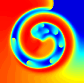
where \(u\) is the membrane potential, \(v\) is a gating variable, and \(a\), \(b\), \(\epsilon\) and \(\delta\) are parameters that determine the dynamics of the system, and \(D\) is the diffusion coefficient that determines the strength of cell-cell coupling. This reaction diffusion system can produce activation waves with periods of refractoriness.
We will consider a square domain and discretize it using a uniform grid. We will represent the grid as a picture, each pixel aligned with the grid. We will use central difference scheme to discretize the diffusion operator in the first equation and we will use the Euler time-stepping for marching the solution.
We can use textures as our data structures and use fragment shaders to update the solution. However, WebGL doesn't allow the same texture to be both the input and output of the solver at the same time. So, we will need at least two textures to march the solution. At each point, one as input and the other as the output.
We assign \(u\) and \(v\) to the red and green channels of the textures. Furthermore, we assign the solution time to the blue channel. We design the fragment shader for time stepping with ample comments for clarity as follows.
#version 300 es
/* &&&&&&&&&&&&&&&&&&&&&&&&&&&&&&&&&&&&&&&&&&&&&&&&&&&& */
/* TIME STEPPING FRAGMENT SHADER                        */
/* &&&&&&&&&&&&&&&&&&&&&&&&&&&&&&&&&&&&&&&&&&&&&&&&&&&& */

precision highp float ;     /* high precision float     */
precision highp int ;       /* high precision integers  */

uniform sampler2D   inTrgt ;/* input texture            */
uniform float       dt ;    /* delta t: time increment  */


/* .....................................................................
   using macros for parameters. consider changing them by uniforms
   and updating them through the graphical user interface as an
   excercise
   .....................................................................
*/
#define diffCoef    0.001   /* diffusion coefficient    */
#define lx          8.0     /* length of the domain     */
#define aa          0.1     /* parameter a              */
#define bb          0.3     /* parameter b              */
#define epsilon     0.01    /* epsilon                  */
#define delta       0.      /* delta                    */

layout (location = 0 ) out vec4 outTrgt ; // output color of the shader

in vec2 cc ;    // Center coordinate of the pixel : between 0-1.

/*----------------------------------------------------------------------
 * main body of the shader
 *----------------------------------------------------------------------
 */
void main() {

    // reading the texture size and calculating delta_x (dx) ...........
    vec2    size = vec2(textureSize( inTrgt,0 )) ;
    float   dx   = lx/size.x ; /* delta x: spacial increment */

    // unit vectors ....................................................
    vec2 ii = vec2(1.,0.)/size ; // unit vector in x
    vec2 jj = vec2(0.,1.)/size ; // unit vector in y

    // calculating laplacian using the  central difference scheme ......
    vec4 laplacian =
            texture( inTrgt, cc-ii  )
        +   texture( inTrgt, cc+ii  )
        +   texture( inTrgt, cc+jj  )
        +   texture( inTrgt, cc-jj  )
        -4.*texture( inTrgt, cc     ) ;

    laplacian = laplacian/(dx*dx) ;

    // extracting values at the center of pixel ........................
    vec4  C = texture( inTrgt, cc ) ;
    float u = C.r ;
    float v = C.g ;
    float time = C.b ;

    // calculating time derivatives ....................................
    float du2dt = laplacian.r*diffCoef + u*(1.0-u)*(u-aa) - v ;
    float dv2dt = epsilon*(bb*u-v+delta)  ;


    // Euler time integration ..........................................
    u += du2dt*dt ;
    v += dv2dt*dt ;
    time += dt ;

    // Pacing at the corner every 200ms ................................
    if ( (int(time)%200 < 1) && length(cc)<0.1 ){u = 1. ;}

    // Updating the output color .......................................
    outTrgt = vec4(u,v,time,1.) ;
    return ;
}
We place the above fragment shader code in <script> tags with the id='tsshader'.
Now, we can define two textures in the main <script> tag for solution time stepping as
var txt1 = new Abubu.Float32Texture(512,512) ;
var txt2 = new Abubu.Float32Texture(512,512) ;
We explained earlier the same texture cannot be both the input and the output of a solver at the same time. To avoid this issue, we define two separate solvers using the above shader. We just swap the input and output textures in these two solvers.
// odd time steps : gets txt1 --> writes txt2 ........................
var tsSolver1 = new Abubu.Solver( {
    fragmentShader : source('tsshader') ,
    uniforms : {
        inTrgt  : { type : 't', value : txt1    } ,
        dt      : { type : 'f', value : 0.05    } ,
    },
    targets : {
        outTrgt : { location :0, target : txt2  } ,
    }
} ) ;

// even time steps : gets txt2 --> writes txt1 .........................
var tsSolver2 = new Abubu.Solver( {
    fragmentShader : source('tsshader') ,
    uniforms : {
        inTrgt  : { type : 't', value : txt2    } ,
        dt      : { type : 'f', value : 0.05    } ,
    },
    targets : {
        outTrgt : { location :0, target : txt1  } ,
    }
} ) ;
Now, if we render tsSolver1 and then tsSolver2, using txt1 we update txt2 and then using txt2, we update txt1. Effectively, we will be marching the solution for two time steps and starting from txt1 and ending in txt1 without having txt1 to be both the input and the output of a solver at the same time.
To visualize the solution, we define a Abubu.Plot2D solver as
var plt = new Abubu.Plot2D({
    target : txt1 ,
    channel: 'r',
    minValue : -.3,
    maxValue : 1.1,
    colorbar : true ,
    canvas : canvas_1
} ) ;
plt.init() ;
We create an infinite loop to march the problem and visualize the soluition by creating the following self calling function:
function run(){
    if (env.running){
        for(var i=0; i < env.skip ; i++){
            tsSolver1.render() ;
            tsSolver2.render() ;
        }
    }
    plt.render() ;
    requestAnimationFrame(run) ;
}
Notice, how a for-loop is placed for updating several time steps before rendering the visualization solver plt. This is due to the fact that plt can be re-launched as often as the screen can be refreshed and that can be a bottleneck in our calculations. Therefore, we choose to skip plotting every time step of the solution to speed up the calculations. The function requestAnimationFrame is a JavaScript function that calls a function when refreshing the screen is complete. By calling the function run in itself we have created an infinite loop that will keep marching the solution as long as the variable env.running is true.
All we need to complete this program, is to have an initialization algorithm. We can also do this using a separate solver that each time it is rendered, it initializes both textures.
#version 300 es
precision highp float ;
precision highp int ;

layout ( location = 0 ) out vec4 outTrgt1 ; // output @ location 1
layout ( location = 1 ) out vec4 outTrgt2 ; // output @ location 2

in vec2 cc ;    // center of pixel location
void main(){
    vec4 outTrgt =vec4(0.) ; // Setting all channels to zero
    if (length(cc)<.1){
        outTrgt.r = 1. ;
    }
    outTrgt1 = outTrgt ;
    outTrgt2 = outTrgt ;
    return ;
}
Assuming this shader is placed in a <script> tag with id='icshader' we can define a solver to utilize this shader as:
var icSolver = new Abubu.Solver({
    fragmentShader : source ('icshader') ,
    targets : {
        outTrgt1 : { location : 0 , target : txt1 } ,
        outTrgt2 : { location : 1 , target : txt2 }
    }
} ) ;
This solver shows you how you can define multiple render targets and update more than 4 color values at the same time. When this solver is rendered, both txt1 and txt2 get initialized.
You can see the complete program at the link below. Also, try to view the source and see if you can figure out the different sections.
Change the skip parameter and observe the difference in solution speed.